
| 일 | 월 | 화 | 수 | 목 | 금 | 토 |
|---|---|---|---|---|---|---|
| 1 | 2 | 3 | ||||
| 4 | 5 | 6 | 7 | 8 | 9 | 10 |
| 11 | 12 | 13 | 14 | 15 | 16 | 17 |
| 18 | 19 | 20 | 21 | 22 | 23 | 24 |
| 25 | 26 | 27 | 28 | 29 | 30 | 31 |
Tags
- 태블로
- konlpy
- numpy
- 데이터분석
- input
- 데이터 분석
- Tableau
- 인공지능
- 크롤링
- Word Cloud
- selenium
- Udemy
- 시각화
- Python
- pandas
- 파이썬
- 데이터
- Okt
- SQL
- 형태소분석기
- pyspark
- scikit-learn
- ionehotencoding
- 머신러닝
- iNT
Archives
- Today
- Total
반전공자
AI - 한글 영화평 데이터 본문
한글 영화평 데이터를 어근만 추출하여 기존의 데이터로 테스트 하였을 때 몇 퍼센트의 정답률을 낼 수 있는가에 대한 실습입니다.
import konlpy
import pandas as pd
import numpy as np
df_train = pd.read_csv('ratings_train.txt', delimiter = '\t', keep_default_na = False)
df_test = pd.read_csv('ratings_test.txt', delimiter = '\t', keep_default_na = False)
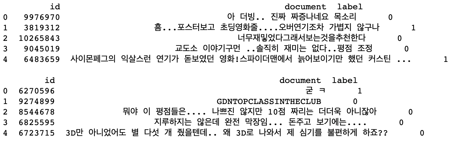
print(df_train.head(n=5), '\n')
print(df_test.head(n=5))
한글 영화평 데이터를 불러온다.
text_train = df_train['document']
y_train = df_train['label']

text_test = df_test['document']
y_test = df_test['label']

print(len(text_train), np.bincount(y_train))
print(len(text_test), np.bincount(y_test))
각각 데이터와 라벨로 분리하여 저장한다.

from konlpy.tag import Okt
twitter_tag = Okt()
def twitter_tokenizer(text):
return twitter_tag.morphs(text)
# 조사, 어미, 구두점, koreanparticle을 제외하는 함수 작성
def twitter_tokenizer_filter(text):
malist = twitter_tag.pos(text, norm = True, stem = True)
r = []
for word in malist:
if not word[1] in ["Josa", "Eomi", "Punctuation", "KoreanParticle"]:
r.append(word[0])
return r
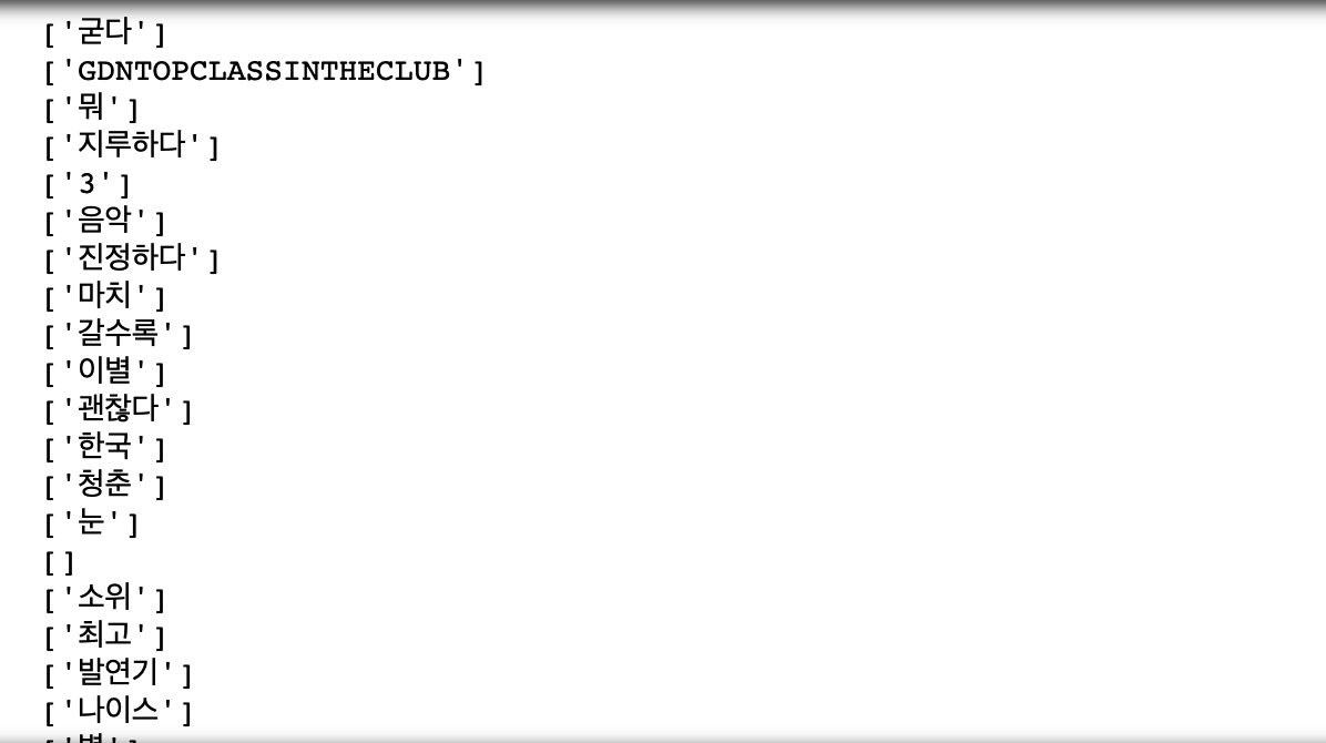
# text_test의 데이터를 twitter_tokenizer_filter함수를 통해 조사, 어미, 구두점, koreanparticle을 모두 제외한다.
for text in text_test:
print(twitter_tokenizer_filter(text))
print(twitter.pos(text_test[0], norm = 'True', stem = 'True'))
print(twitter.pos(text_test[2], norm = 'True', stem = 'True'))

이전의 데이터에는 그냥 줄글로 평이 저장되어있었는데
조사, 어미 등을 제외한 후에는 남은 단어들이 각각 리스트로 저장되어있다.
from sklearn.feature_extraction.text import CountVectorizer
from sklearn.feature_extraction.text import TfidfVectorizer
# corpus에 train 데이터를 옮겨놓고 Tfidf Vectorizer를 실행한다.
corpus = text_train
vect1 = CountVectorizer().fit(corpus)
tf = vect1.transform(corpus)
# bow의 일부를 출력
feature_names = vect1.get_feature_names()
print("Term: {}".format(feature_names[500:510]))
# tfidf Vectorizer를 실행한 결과 일부를 sparse matrix 형태로 출력
vect2 = TfidfVectorizer().fit(corpus)
tfidf = vect2.transform(corpus)
print(tfidf[500:510])
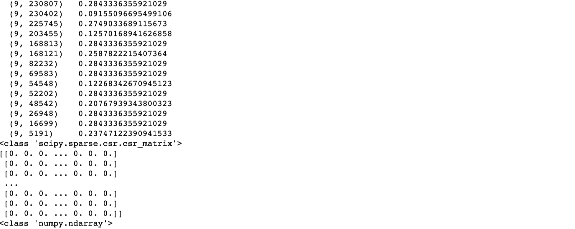
print(type(tfidf))
# 일부를 array 형태로 출력
print(tfidf.toarray()[500:510])
print(type(tfidf.toarray()))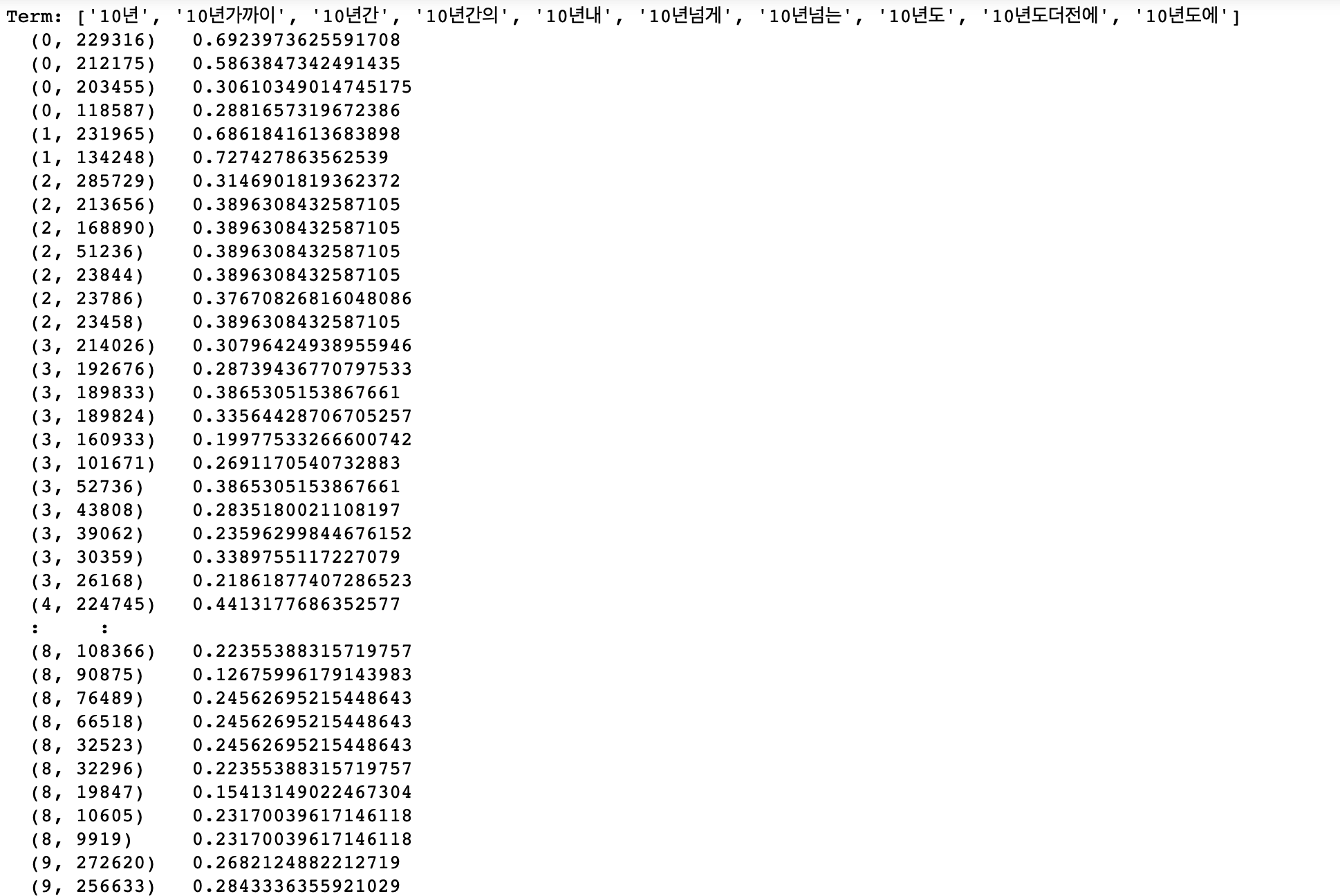
import konlpy
import pandas as pd
import numpy as np

from sklearn.feature_extraction.text import CountVectorizer
from sklearn import metrics
from sklearn.naive_bayes import MultinomialNB

from konlpy.tag import Okt
# 위에서 작성했던 함수인 twitter_tokenizer를 활용하여 text_train을 fit 시킨다.
vect = CountVectorizer(tokenizer = twitter_tokenizer).fit(text_train)X_train = vect.transform(text_train)
clf_mult = MultinomialNB().fit(X_train, y_train)X_test = vect.transform(text_test)pre = clf_mult.predict(X_test)# 정답률 출력
ac_score = metrics.accuracy_score(y_test, pre)
print("정답률 = ", round(ac_score,2)) # 85%의 정답률, 소수점 둘째자리까지 잘라서 출력
# 알파값이 얼마일 때 정확도가 가장 높은지 찾아보자.
nb = MultinomialNB(alpha = 1.2)
nb.fit(X_train, y_train)
pre = nb.predict(X_test)

ac_score = metrics.accuracy_score(y_test, pre)
print("정답률 =", ac_score)

nb = MultinomialNB(alpha = 0.7)
nb.fit(X_train, y_train)
pre = nb.predict(X_test)

ac_score = metrics.accuracy_score(y_test, pre)
print("정답률 =", ac_score)
nb = MultinomialNB(alpha = 0.5)
nb.fit(X_train, y_train)
pre = nb.predict(X_test)

ac_score = metrics.accuracy_score(y_test, pre)
print("정답률 =", ac_score)
nb = MultinomialNB(alpha = 0.6)
nb.fit(X_train, y_train)
pre = nb.predict(X_test)

ac_score = metrics.accuracy_score(y_test, pre)
print("정답률 =", ac_score)
## alpha = 0.6일 때가 가장 최적의 정답률이다.
# 알파 값 별 정답률 계산하여 리스트에 저장하는 함수
# 알파값 별 정답률을 계산하고 각각을 리스트형태로 저장하는 함수 작성
score_a = []
alpha = []
def score_cal(num):
    nb = MultinomialNB(alpha = num)
    nb.fit(X_train, y_train)
    pre = nb.predict(X_test)
    ac_score = metrics.accuracy_score(y_test, pre)
    print(ac_score)
    score_a.append(ac_score)
    print(num)
    alpha.append(num)
score_cal(0.1)
정답률과 알파값이 같이 출력된다. 그 뒤에서는 리스트에 각각의 값을 저장하고 있다.
# 0.1 부터 5.0까지의 수를 리스트 형태로 저장해 놓는다.
al_li = np.arange(0.1,5.1,0.1)
# 위에서 만들어 놓은 범위 별로 for문을 통해 함수 돌리기.
for i in al_li :
score_cal(i)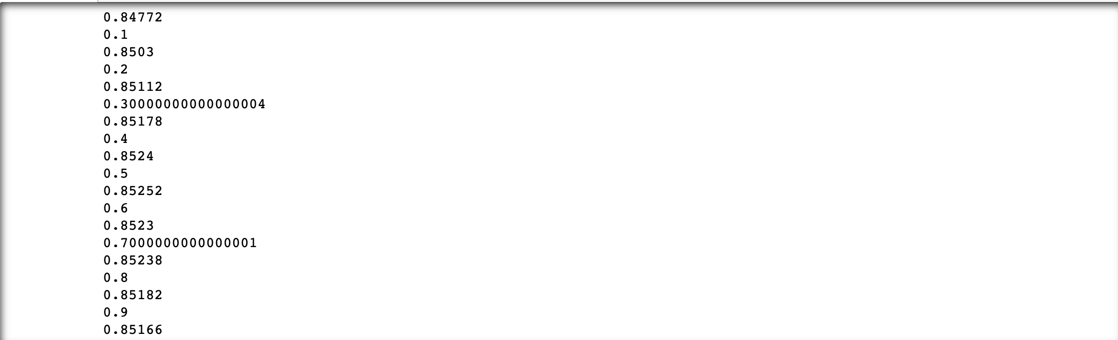
# 알파값과 그에 따른 정답률이 모두 리스트 형식으로 저장되었음을 알 수 있다.
print(score_a)
print(alpha)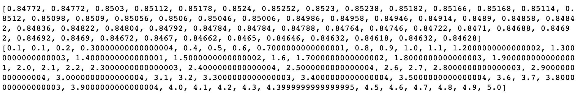
첫번째 리스트는 정답률
두번째 리스트는 알파값
from matplotlib import pyplot as plt
import numpy as np

# x에 알파, y에 정답률 저장
x = alpha
y = score_a

# 그래프 그리기
plt.title('alpha - score')
plt.xlabel('alpha')
plt.ylabel('score')
plt.plot(x,y)
plt.show()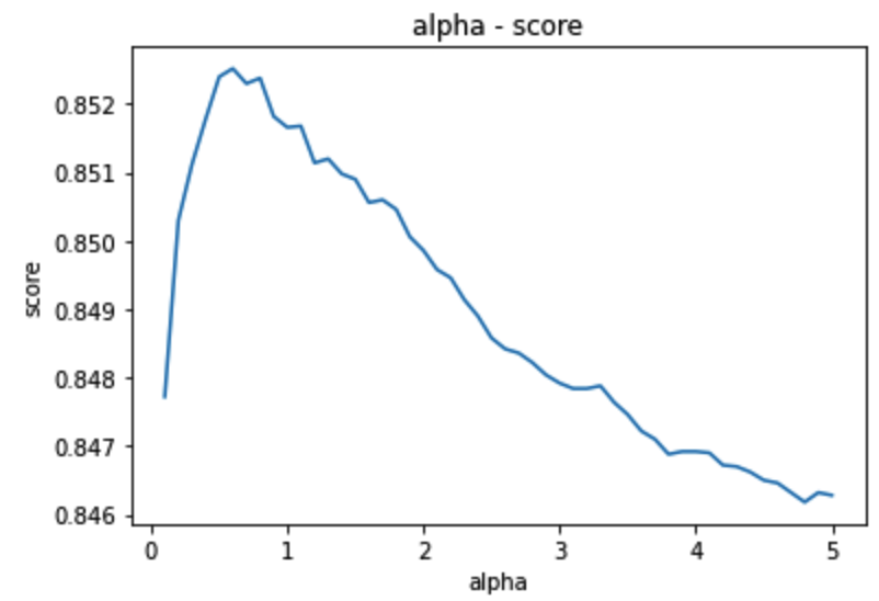
'데이터분석 > 데테_인공지능' 카테고리의 다른 글
| Octave 기본문법 (Range, data structure (0) | 2021.06.05 |
|---|---|
| Octave 기본 문법 (class(), Matrics) (0) | 2021.06.04 |
| WordCloud (0) | 2021.05.07 |
| Nominal Attribute (LabelEncoder, fit, transform) (0) | 2021.04.28 |
| Data Preprocessing (scikit-learn, Scaling(minimax_scale, fit_transform) (0) | 2021.04.08 |