
| 일 | 월 | 화 | 수 | 목 | 금 | 토 |
|---|---|---|---|---|---|---|
| 1 | 2 | 3 | ||||
| 4 | 5 | 6 | 7 | 8 | 9 | 10 |
| 11 | 12 | 13 | 14 | 15 | 16 | 17 |
| 18 | 19 | 20 | 21 | 22 | 23 | 24 |
| 25 | 26 | 27 | 28 | 29 | 30 | 31 |
Tags
- 시각화
- selenium
- ionehotencoding
- konlpy
- Udemy
- 파이썬
- Tableau
- 머신러닝
- 데이터
- 데이터 분석
- 형태소분석기
- 크롤링
- 인공지능
- iNT
- Python
- pyspark
- 데이터분석
- numpy
- 태블로
- scikit-learn
- SQL
- pandas
- Word Cloud
- input
- Okt
Archives
- Today
- Total
반전공자
R - 난수, 분포함수 본문
# 평균 0, 표준편차 10인 정규분포로부터 난수 100개를 생성
rnorm(100,0,10)

# 많은 수의 난수 생성 후 밀도 그림 그리면 데이터 분포 파악 가능
plot(density(rnorm(100000,0,10)))

pnorm(0)
[1] 0.5
qnorm(0.5)
[1] 0
[ 확률 밀도 함수 활용 ]
12세 미만인 어린이가 보통 하루에 마시는 물 양의 평균이 7.5, 표준편차가 1.5인 정규분포를 따른다 가정,
(1) 어린이가 4리터 이하의 물을 마실 확률?
x = seq(0,16, length=100)
y = dnorm(x, mean=7.5, sd=1.5)
plot(x,y,type="l",
	xlab="Liters per day",
    ylab="Density",
    main="Liters of water drunken by school children < 12 years old")

# 4리터 이하의 마실 확률 : Lower tail
pnorm(4, mean=7.5, sd=1.5, lower.tail=TRUE)
[1] 0.009815329 # 결과
(2). 어린이가 8리터 이상의 물을 마실 확률은 얼마? 정규곡선에 해당 영역을 지정하여 색칠하기.
plot.new()
plot(x,y,type="l",
	xlab="Liters per day",
    ylab="Density") # 첫번째 그래프

# 8리터 이상 물을 마실 확률
lower = 8
upper = 15

# 8~15 사이의 값을 모으기
i=x>lower & x<upper
polygon(c(lower, x[i], upper), c(0, y[i], 0), col="red") # 해당영역 색칠
abline(h=0, col="gray") # 두번째 그래프

# 확률계산
pb = round(pnorm(8, mean=7.5, sd=1.5, lower.tail=FALSE),2)
pb
pb.result = paste("Cumulative probability of a child drinking > 8L/day", pb, seq=":")
title(pb.result) # 그래프에 제목 추가


[ 기초 통계량 ]
> mean(1:5) # 평균
[1] 3

> var(1:5) # 분산
[1] 2.5

> sd(1:5) # 표준편차
[1] 1.581139

> fivenum(1:11) # 최저, Q1, 중앙, Q3, 최고
[1]  1.0  3.5  6.0  8.5 11.0

> summary(1:11) # fivenum + mean
   Min. 1st Qu.  Median    Mean 3rd Qu.    Max.
    1.0     3.5     6.0     6.0     8.5    11.0

> x = factor(c("a","b","c","c","c","d","d")) # factor형 자료 생성
> x # 자료 형태 보여줌
[1] a b c c c d d
Levels: a b c d # 총 네가지의 자료가 들어있다.

> table(x) # 빈도 체크
x
a b c d
1 1 3 2

> which.max(table(x)) # 빈도 가장 높은것은?
c
3

> names(table(x))[3] # table에서 세번째에 위치하는 데이터?
[1] "c"
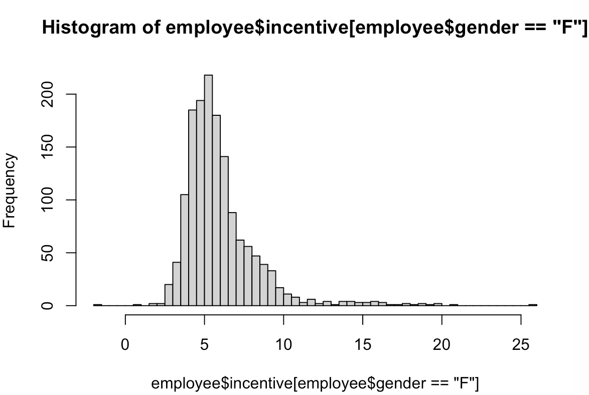
[ employee_ex.csv 활용 데이터 분석 ]
employee <- read.csv("employees_ex.csv")

hist(employee$incentive[employee$year==2007], breaks=50)
hist(employee$incentive[employee$year==2008], breaks=50)
hist(employee$incentive[employee$gender=="F"], breaks=50)
hist(employee$incentive[employee$gender=="M"], breaks=50)
hist(employee$incentive[employee$negotiated==FALSE], breaks=50)
hist(employee$incentive[employee$negotiated==TRUE], breaks=50)


install.packages("propagate")
library(propagate)
set.seed(275)
observations = rnorm(10000,5)
disTested=fitdistr(observations)
* 정규분포에 fit 된 것 같다.
'데이터분석 > R' 카테고리의 다른 글
| R - [ 실습: 수면제 효과도 분석 ]: sleep 데이터 활용 (0) | 2021.05.13 |
|---|---|
| R - 분석방법 (카이제곱, 피셔검정, KS검정, Shapiro 검정, t-test) (0) | 2021.05.12 |
| R - welfare.csv, 결측치 대체 함수 작성 (0) | 2021.05.09 |
| R - Airquality (0) | 2021.05.09 |
| R 통계분석 (5) 분석과제 ( mpg data) (0) | 2021.04.08 |